
The geometry of nonergodic composition
Implicit Bayesian inference, made explicit
Introduction
Perhaps the defining feature of LLM pretraining data is its heterogeneity. The training corpus spans not only the collected and varied textual works output by the whole of humanity, but also those generated by machines, data collection devices, and more. Such a large and varied corpus is often appealed to as an explanation for the abilities of modern LLMs1. But the statistical structure of data created by a diverse set of generators also implies a particular computational structure for the next token prediction task, and, as we will see, for the geometric arrangement of the internal activations in LLMs.
In order to understand the structure of the next token prediction task over data generated from many different sources, and its implications for the geometric structure of activations in neural networks, we will:
- Start by introducing the concept of nonergodicity, which is an important property of LLM training data. Nonergodicity formalizes the notion of a generator of data made of many sources.
- Derive the belief geometry that the prediction task over such data implies: per-source belief geometries whose magnitude scales in accordance with how strongly the context supports each component. This gives rise to the telescoping geometric structures shown in this post, and to feature geometry that is eventually sparse and multi-dimensional.
- Treat this geometry as a falsifiable prediction. If a network represents beliefs linearly, as we have found before[5], the geometry of its activations should take this form. By using data with known mixture structure and known per-component geometry, we are able to predict and then observe a transformer building that geometry.
We are excited about these results because nonergodicity is a fundamental statistical aspect of real pretraining data. It is, in some sense, the structure that makes in-context learning both necessary and powerful. Xie et al. [6] argued that when pretraining data is a mixture of latent generative concepts, in-context learning should be thought of as the model implicitly performing Bayesian inference over those concepts. In Riechers et al. [7] and Shai et al. [5], we showed that next-token pretraining forces this kind of inference even within a single concept. Nonergodic data calls for both at once. Here, we investigate the specific computational and geometric implications of this type of hierarchical inference.
LLM Training Data is Nonergodic
Consider a natural language sequence beginning with Do not make…. This ambiguous opening reveals little about the source.
- my mistake, buy the bigger one. edit: I know, please stop DMing me. a redditor
- adjustments while the unit is connected to power. an appliance manual
- too much of what M. said at dinner. You always do this. a private journal
- the reader hunt through the appendix. Also, this appears in my 2019 paper. Weak reject. referee #2
These four completions share a prefix, but they do not share a future. Note how each continuation gives information about the generator of that data sample, in this case, a Redditor, an instruction manual, etc. These different sources create token sequences with different correlation structure, which is revealed through additional context. The language of a document, the genre of a story, and the identity of a speaker are all initial choices that jointly constrain the subsequent tokens. In the language of stochastic processes, these situations correspond to nonergodic compositions: mixtures of distinct generative processes, where the identity of the active process is fixed at the start of each sequence generation and never revisited. Much of our previous work has dealt with inference over a world model composed of a single generator; here we extend the discussion to include the meta process of inference about which of multiple generators in the world we should be modeling at all.
In the rest of this post, we will explain how the theory predicts a telescoping geometric structure for beliefs over this kind of data, and show some initial results consistent with the fact that transformers represent that geometry in their activations when trained on nonergodic data.
Two coins: the simplest example of a nonergodic process
In order to understand inference over such nonergodic data sources, we will start with the simple example of data generated from one of two coins. Imagine you know that I have two coins, coin and coin , each of different fixed biases. I secretly choose one at random and start flipping it. You see only the outcomes: H, T, H, H, T, H, H,…. Your task is to predict the next heads or tails. To do that, it would be useful if you could figure out if it was coin or coin that was responsible for the flips you’ve seen so far. At first, you have no idea which coin is being flipped, and all you have is your prior: “it could just as easily be either coin”. But as flips accumulate, the frequency of heads tilts toward one of the two biases, and you will become more confident about which of the coins is active. That process is the process of sequentially updating your posterior to a strong belief about the world: “I’m pretty sure I know which coin it is.”
This is the simplest nonergodic composition; the coins are stand-ins for more generic ergodic components2 that may themselves carry nontrivial latent structure. We will tackle that case momentarily, but here we have two memoryless3 components. The only memory is a hidden “which coin” latent that is set once for each sequence generation and never changed. This choice is hidden because you never see the initial selection directly, but Bayesian inference eventually resolves your uncertainty from observation statistics alone.
Together, the two coins can be thought of as one generator with two hidden states and no way to move between them. Once you know that one of the coins generated the sequence, there is nothing more to know, so your knowledge of the system is fully determined by your belief about which coin is generating the data, which is a point on a segment that slides toward one end as evidence accumulates.
You can try this yourself: flip as many times as you like to gather evidence, set your belief about which coin is responsible for generating the data, and then reveal the Bayes-optimal posterior and the coin.
generated the sequence
For these coins, the optimal Bayesian posterior can simply be written down given a sequence of observations; the counts of heads and tails are all it needs (you might remember this from your statistics class). In our case, we have the two coins, and , with biases and and a prior over which one is active. After heads and tails, the posterior on coin is:
The form of this equation shows one of the fundamental lessons of this post. When formally answering the question “what is the probability that coin A generated the sequence?”4 the numerator only depends on information about coin A: coin A’s own likelihood times coin A’s prior. It notably does not depend on information about coin B! The denominator, in contrast, normalizes this numerator by a sum that depends on both coins, and thus couples the belief in coin A with information about both coins. We will see that the form of this belief update, containing a part that has to do with each component independently, and then normalized by a part that has to do with all components, is general.
For the case of the coins, the order of the flips doesn’t matter at all. This is not general, and is atypical of the real world. Most environments that we need to identify have sequential structure. I not you kid. Sorry, rather: I kid you not. Order matters.
In the more general case, the identity of a source lives in the detailed correlation structure of how its tokens follow one another, not just in counts of tokens. A Reddit thread, for example, has many hidden states — what account has replied and what was said are directly observable, but not whether the person behind the account is hungry, or tired. Once components have internal structure, just counting current symbols is no longer enough. We need the general answer to the question the coins raised: what, exactly, must you remember about the past in order to best predict the future? The answer to this is the belief state.
Nonergodic Generators of Data and the Task of Prediction over them
To concretize this into a falsifiable theory, we will need to formalize a general notion of a generator of data composed of many different sources. Each source should have its own internal latent structure, and should generate sequences of tokens. In addition, multiple sources need to be able to be composed in such a way that is consistent with the notion of one source being active, or another source, but not more than one simultaneously.
In the following section, we quickly review the mathematical structure of Hidden Markov Models (HMMs) as latent generators of token sequences, the task of prediction over those sequences, and the corresponding belief geometry associated with that prediction task5. This section is all a review of our earlier work [5], but is necessary to get to Section 4 where we use HMMs as building blocks for nonergodic composition of generators, and study the geometric structure of prediction over those.
HMMs as Latent Generators of Token Sequences
We are trying to capture the situation relevant to the task of prediction over sequences of data, especially when the data is generated by processes that are hidden to the predictor. As in our earlier work, we will use the framework of Hidden Markov Models (HMMs) as our fundamental generator component.
An HMM has a set of hidden states, , and emits tokens from a vocabulary . Its dynamics are given by one transition operator per token, , whose entry is the probability that the generator moves from hidden state to hidden state and emits as it does so. These operators define both how the hidden states move and also how the state dynamics relate to token emissions. You may remember Mess3, the 3-state HMM shown below on the right, from our earlier work.
CCACCCCAABAA…
Natural language is of course more complicated than these examples, but notably any stochastic process6 can be generated by some HMM.
The Task of Prediction and Belief State Geometry
Despite the name (GPT stands for generative pretrained transformer), transformers are actually (pre)trained to predict, not generate. A predictor observing sequences of tokens and trying to predict the next token cannot directly see the hidden state of the generator. What it can do is keep a belief , a probability distribution over the hidden states, and update it with each token. As discussed in our previous work, an optimal predictor will update its belief, upon seeing a token , from to , according to Bayes’ Rule.
BCC.
These belief states are vectors that live in a probability simplex. The set of belief states that are reachable from the sequences a generator creates thus has a geometry, the belief state geometry. For instance, in the case of Mess3, there are an infinite number of distinct belief states, that arrange themselves in the probability simplex as a fractal.
Importantly, the information a belief state contains is everything the past tells you about the future; it is the general answer to the question the coins raised. For a coin the belief over its single state is trivially the number one, which is why counting heads and tails was all there was to do. The posterior over which coin was a belief of a different kind, a belief about which generator is active. As we will now see, in general a predictor has to carry both types of information.
Nonergodicity, Prediction, and Telescoping Geometry!
We now have all the pieces needed to create a generator composed of multiple sources/components. The high level approach will be to design a single HMM whose hidden states are the hidden states of all the components put together, and whose dynamics never move between components. The coin game from earlier is a simple example of this: pick a coin, then generate a sequence using only that coin. After we have an HMM that generates nonergodic data, we will figure out the geometric consequences for prediction.
Nonergodic Composition
The mathematical move to create generators of nonergodic data, called nonergodic composition, will be to compose component HMMs via the direct sum. We find that it is often helpful to see both the general theory and an example to keep intuition grounded, so we encourage you to flip between the tabs below.
General theory
Given component HMMs , the nonergodic composition is a single HMM whose token-labeled transition matrices are the direct sum of the components’ matrices :
The block-diagonal structure is the key property: since the off-diagonal blocks are zero, a state in block can never transition to block . The process is permanently confined to whichever block it starts in 7.
We also need to compose the initial states, . Each sums to 1 within its own component, but not across components. So to compose them we need to choose a weight for each component, with , which is the prior probability that component is the one generating the data. The initial state vector of the composition is then the concatenation of the components’ initial vectors, each scaled by the weight on its component,
Mess3 example
Let us consider the nonergodic composition of two Mess3 generators, each acting as a distinct source of token sequences. We will call them Component and Component . Each Mess3 will have different hyperparameter settings, as shown below. To make a single generator out of these components, in which every sequence is generated either by or by with 50/50 probability, we arrange the transition matrices of the two components in block-diagonal form8.
This composite HMM is another HMM, a latent generator of sequences of tokens. Note that because the transition probabilities associated with one component always have zero probability of transition to any state in the other component (the off-diagonal terms are all zero by construction), it is impossible for the generator to move between components, once it has started in one.
Belief Geometry over Nonergodic Data
Next, we apply the belief update rule to such a composition of ergodic components. We will see that while the generator is permanently confined to whichever block it starts in, an observer’s guess about which component is active is not [8]. Like guessing the hidden coin from a sequence: the true coin is always the same, but as flips accumulate you change your belief about which one it is. In the belief geometry, this ends up coupling geometric structures associated with each component in a particular way.
The belief updating rule is the same as for a single component HMM,
but now both the initial state and the transition operators have block structure:
Let’s take a look at the belief state after a single token emission. Because the off-diagonal blocks of are zero, the numerator of the belief update acts block by block:
Each component’s initial belief gets multiplied by its own operator, as if it were the only generator. The denominator of the belief update is a normalization, which sums over all entries of the numerator, and thus couples the belief updating across the components by a scalar. A small bit of algebra9 shows that we are again left with a concatenation of per component beliefs each scaled by a scalar with . The resulting belief state, and indeed all reachable belief states (due to the recursive nature of belief updating), can be expressed this way. We can always decompose a belief as
Because of this, our interpretation of the initial state carries over to all belief states, with the mixture prior becoming a per-component mixture posterior . In short: the belief is a distribution over all components’ hidden states that can always be expressed in terms of the probability that the predictor puts on component , and the belief over the states of component , conditioned on being in that component.
wA = 0.50 wB = 0.50
From this we can see something important about the belief geometry. The beliefs of a nonergodic composition live in a simplex whose dimension is set by the total number of hidden states across all the components. For our two 3-state HMMs, that is 6 states, so the 5-simplex. From that 5 dimensional space, we can project the belief onto the coordinates of any single component, giving . This is a point in a simplex, but shrunk toward the origin by the weight . The are not independent from each other: they sum to one. So, as the belief puts more weight on one component, its simplex grows in magnitude, and the others shrink towards the origin. Thus, the projection gives the belief geometry a telescoping effect. Above, we show where the belief vectors can live when looking at this projection for two arbitrary 3-state HMMs, for any given . The toggles show and hide the specific fractals for a nonergodic composition of two Mess3s.
The result is that components that explain the observed data well accrue weight; components that don’t, lose it. Belief updating over such a composition has a characteristic signature: eventually sparse multi-dimensional features. Early in context, several components carry non-negligible weight ; as we see more tokens and evidence accumulates we expect for the true component , and the geometry to collapse onto the active block only.
Does this geometry show up in trained models?
The framework above predicts a specific geometric structure for the belief geometry associated with prediction on nonergodic token sequences. When a transformer is trained on next-token prediction over such data, can we find that geometry in its activations?
Here we show our initial positive results. To test this in a transformer we use a nonergodic composition of two Mess3 generators. Mess3’s belief states form a fractal that fills the simplex, so the nonergodic composition of two Mess3 components should give two fractal-filled cones, each telescopically scaling with the weight on its component.
The interactive figure below shows the ground truth belief geometry, which serves as a nontrivial falsifiable prediction for what we should find in the transformer activations. The full beliefs live in 5 dimensions, and what is shown below are two 3D projections from the 5-simplex to the belief entries associated with each component. Drag either panel to rotate both, and use the ℓ slider to move through the context.
We trained transformers on a nonergodic composition of two Mess3 generators. Our theory predicts that the activations should track the belief states. Because we have ground-truth access to the generator, we know the exact belief vector associated with each context position. A linear map fit from the residual stream to these ground-truth belief states recovers them on held-out contexts with R² ≈ 0.985 (compare to an untrained network, which is at ≈ 0.45), and the predicted geometry appears in the residual stream over training:
We see our two telescoping cones, one for each component, scaling with the posterior weight on that component. This emerges as a direct consequence of pretraining on next-token cross-entropy alone. Nothing in the training objective tells the model directly about components, belief vectors, or simplices. The color here encodes the entropy that a Bayesian observer would have over which of the two components is active, given the context that led to that activation. The middle yellow region corresponds to contexts that are well explained by either component, and the states of maximum certainty are the darker tips and faces of the cones.
Below, you can explore the geometry of the converged model’s activations. The left panel is the cumulative variance explained by PCA of the final layer activations, drawn separately for contexts generated by each component ( and ); the two right panels show those same activations passed through the learned linear map to the predicted geometry. You can filter activations by ground-truth posterior entropy or by context position. Try dragging the maximum posterior entropy slider down toward 0. This means keeping only contexts where the evidence supports committing largely to one component. We see that the CEV curves climb faster, meaning the activations effectively fill fewer dimensions as the model hones in on a single component. Meanwhile, in the scatter plot, the cone for the now-unlikely component collapses toward the origin. Filtering to late sequence positions tells a similar, but noisier story. Additional context is increasingly likely to support just one component or the other, but it is also possible to observe long sequences that have similar likelihood under either component, or are even flat out misleading (perhaps you ran into some of these in the coin game?).
Did it have to be this way?
The way we derived the nonergodic belief geometry, it may seem almost as if there was no alternative for what the neural network should represent 10. In light of this, it is worth explicitly pointing out that the predicted geometry is not something that just has to be present for the model to output correct next-token probabilities. This representation manifestly carries more distinctions between contexts than are implied by their differences in next-token prediction. While the beliefs live in 5 dimensions (a distribution over 6 hidden states), the next-token distribution lives only in 2 dimensions (a distribution over 3 possible tokens). Of course, this geometry does perfectly contain the distribution over the next token– but it also represents distinctions in the token after, the 10th token, and the joint probability distribution of the 3rd and 11th tokens conditioned on the 9th. It fully contains all distinctions that can be made between distributions over the future, yet it emerged only by looking one token ahead.
See the plot below, which shows the first three principal components of the 5-dimensional predictive geometry (right), colored by the associated next-token distribution. A small region in the next-token simplex (left) can correspond to significantly different parts of the full-future predictive geometry.
You can scroll around the next-token simplex yourself. You will see that some regions in the next token simplex correspond to unambiguous distributions over the future and other next-token distributions permit many different distributions over the full future.
We note that these canonical low-dimensional representations emerge most cleanly when we initialize network weights to be small, perhaps placing the network in the “rich” feature learning training regime studied in deep learning theory as opposed to the “lazy” one [9, 10].
Parting thoughts
The next token prediction task over nonergodic data requires two levels of inference: figuring out which generator is currently active, while also tracking what state that generator is in. One geometric implication for the activations of neural networks is a per-component projective embedding of the belief geometry with each component’s scale being the posterior weight accorded that component. With this geometry as a falsifiable prediction, we trained transformers on nonergodic compositions, and found this geometry linearly embedded in the residual stream.
Real data is made of many more sources than two, and they will overlap in their structure to different, and quite complicated, degrees. Some components will share most of their structure and differ in a few probabilities; others will share almost nothing; many will sit somewhere in between11. Taken together, we should expect a rich, hierarchical inference process to emerge from that: weights over components, weights over groups of components that look alike, and within each, the component’s own belief updating. This is one way to see why pretraining on such data produces in-context learning [7].
In closing, let’s revisit the humble coin. Some data is closer to a bag holding infinitely many coins: you draw a bias from the continuum and start flipping (the problem Laplace solved in 1774); the sum over coins in the Bayesian updating equation becomes an integral, the finite set of weights (one for each component) become a continuum of weights, and the telescoping picture would need infinitely many cones. Yet, the formula for the weights would still only ever consults two numbers, the counts and , so the distinct beliefs an observer can hold about the future still form a finite-dimensional predictive geometry, described by two parameters: an estimate (the fraction of heads) and how certain it is (the total number of flips). Whether a model stores such beliefs or computes them from running tallies, and what that means for a continuum of memoryfull components with nontrivial internal structure, and for generalization, is the subject of a post to come.
Our story supports a refinement to the picture of transformer representations as sums of sparse one-dimensional features that motivates sparse autoencoders [12, 13, 14]. For data with nonergodic structure, the right ansatz seems instead to be sparse dense subspaces — multi-dimensional geometries that correspond to inference-time Bayesian updating over an underlying world model that includes mutually exclusive12 parts. The model uses many dimensions while a given component is in play, but eventually only a few components carry weight at any given time. Sparsity at the component level, density within each component. The same machinery extends naturally to compositions with internal factorization (each component itself a product of more elementary parts), and it predicts that models trained on factorizable data should discover those parts, represent them in correspondingly factored subspaces [15], and also simultaneously keep track of the meta dynamic over the components.
This picture, of transformer representations as a sparse sum of points within multidimensional subspaces of activation space, is consistent with recent work extending the “linear representation hypothesis” [12] to accommodate observations of multidimensional features in language models [16, 17]. These works suggest that neural network activations be modeled as sums of multidimensional features, whose value is represented as a point in subspaces of dimension greater than 1, but where most such features don’t have a defined value (or have value ~0) on most activations (they are sparse). We find this picture emerges naturally from theory as a consequence of performing prediction over a process consisting of nonergodic components.
Appendix
Acknowledgments
This post draws on joint work at Simplex on the geometry of belief states in nonergodic sequence tasks. Particularly, we thank Javan Tahir, Casper Christensen, Loren Amdahl-Culleton, and Andrew Jun Lee for helpful discussions; Eric Michaud, Jasmina Urdshals, and Selma Maizioud for helpful comments on this blog; and Eric Michaud for input on our discussion of sparse autoencoders and the multidimensional linear representation hypothesis.
A version of this problem has served as a take-home question for Simplex job and MATS applications; the theory and results presented here were developed beforehand and are independent of any applicant work. We thank the applicants for the care and creativity they brought to the problem.
We used LLMs (Opus 4.5+, Opus 5.0, and Fable) to design and run experiments, design this blog, and draft this post. Most prose in this version was written by the authors. We take all responsibility for the content.
The Mess3 process
The Mess3 process [5, 18] has three hidden states , and three observable tokens .
The process is defined by two parameters, and , with dependent quantities and . The two components used throughout this post are drawn from this family: the first uses and the second uses .
The labeled transition matrices are:
Training details
Data. Sequences are drawn from the nonergodic composition of the two Mess3 components defined above, mixed with equal weight. Each training sequence begins with a BOS token and then stays inside a single component for all 127 subsequent tokens; the two components share the same three-token alphabet, so no individual token reveals which component is active.
Model. A four-layer decoder-only transformer (TransformerLens HookedTransformer): , four attention heads of dimension 32, gated GELU MLPs of width 512, RMS normalization, rotary position embeddings, context length 128, and a vocabulary of four tokens (three emissions plus BOS). Weights are initialized from a Gaussian with standard deviation 0.02, about smaller than the TransformerLens default of .
Optimization. AdamW (, no weight decay) at a constant learning rate of , with batches of 512 sequences.
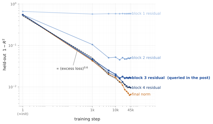
Metrics over Training. By step 10,000 the model’s next-token distribution sits within a few nats per token of the optimal loss, and at the step-45,000 checkpoint used for the figures the gap is about . While the loss is falling, the regression error tracks it: drops roughly as the excess loss to the power in every layer past the first (every layer in which we find a belief representation). Once the loss reaches its floor, each layer settles onto a floor of its own, later for deeper layers. The animations in this post and the activation explorer use the residual stream after the third of the four blocks, where a linear map recovers the weighted belief vectors with held-out ; at the output of the final transformer block, it reaches .
Generators of Data and the Geometry of Beliefs
The three subsections below restate (at two levels of formality which you can toggle between) the mathematical machinery of our work [5]: hidden Markov models as latent generators of token sequences, belief updating as the structure of prediction, and the geometry of those beliefs.
Fundamentally we are trying to capture the situation relevant to the task prediction over sequences of data, especially when the data is generated by processes that are hidden to the predictor. As such, whatever our formal notion of a generator is, it should have an internal latent space that is hidden from the predictor, a set of rules for how that latent space changes through time (or context position), and a set of rules for how changes in the latent space relate to the observations (or tokens) emitted.
Everything below also holds for generalized HMMs (GHMMs), in which the transition operators may carry negative entries and the predictive vector need not be a probability distribution. Finite GHMMs represent a strictly wider class of processes than finite HMMs — the non-classical geometries of our companion post — but every example here is an ordinary HMM.
In the following sections, we present this work at two levels of formality. If you are interested in the concepts without necessarily the formal mathematics, we suggest choosing the Worked example tab. If, instead, equations are what spark joy in you, choose the General theory tab.
HMMs and their transition operators
General theory
HMMs are an extremely flexible model class: with enough hidden states, essentially any distribution over token sequences can be represented by one. An HMM is defined by the tuple
where is the token alphabet, is the latent space, is an initial state vector, and each is the operator describing latent dynamics for emission . The net transition operator must have a right eigenvector with unit eigenvalue. We can then interpret the dynamical systems latent space as carrying a conserved probability mass for which is the integrator. This means we can interpret the probability of any token sequence as being expressed by
It is in this sense that we say that an HMM generates a stochastic process.
Worked example
Consider token sequences of the form 0, then 1, then a random bit, and repeats:...0 1 R 0 1 R …. Importantly, sequences can start at any of the three phases. We will call this the Z1R process (for “zero one random”). Here, we are interested in a latent generator of such data. As discussed above, it should have latent states, and dynamical rules telling us how those latent states change through time, and how those changes relate to token emissions.
One such generator for this particular data is a hidden Markov model (HMM). It has three latent states: , , and , which can be represented by circles in a graph as shown below.
Graphical representation
arrow from state iS0S1SR to state jS0S1SR: token x01, probability p01½
Algebraic representation
T(0) =to statefrom stateS0S1SRS0010S1000SR½00T(1) =to statefrom stateS0S1SRS0000S1001SR½00
T(x01)iS0S1SR jS0S1SR = P(st+1 = jS0S1SR, xt+1 = x01 | st = iS0S1SR)= 0= 1= ½
Sequences of tokens are generated by starting in a particular state (or a distribution over states), then following the arrows according to the probabilities on them. Upon choosing an arrow, the system moves to another latent state (which could be the same one), and emits a token, .
One can represent this system algebraically as well, as a set of token-labeled transition matrices, with one matrix, , per token. The entries of these matrices, , are the probability that the system, sitting in state , takes the arrow to state and emits the token . In the figure above on the right, you can see the transition matrices for an HMM that generates the Z1R process.
The only other part needed to define an HMM is the initial state, denoted . In general this can be any probability distribution over the latent states of the system. When the HMM is generating a sequence, you can think of its starting state as being sampled from this initial state13.
Prediction Over Data Generated by HMMs
In the previous section we discussed generators of token sequence data. What is the computational structure of the prediction task, relative to the structure of the latent generator of the token sequence data?
Here we review the answer we established in our previous work: the information that a predictor must represent in order to take in sequences of token and predict future token sequences is given by beliefs, , over the hidden states of the latent generator of that data.
General theory
We are interested here in the task of prediction of future token sequences given observations of past token sequences. Formally, the conditional probability of any future sequence given the observed context is
We call the vector encoding the past information the predictive vector (for an HMM, where it is a probability distribution over the hidden states, this is the belief state ):
This vector is the general answer to the question the coins raised. For the memoryless coins it collapses to the head/tail counts; in general it is everything the past tells you about the future, and nothing more.
Token by token, the same vector updates by one matrix multiplication and a renormalization,
where the denominator is the probability the observer assigned to the token that just arrived — its next-token prediction.
Because the conditional probability above can be written as
iterating this update rule from recovers exactly this closed form.
Worked example
We are interested here in the task of prediction of future token sequences given observations of past token sequences. Intuitively, if we see a sequence of tokens from Z1R in context, like 0110, we would do well to figure out which of the latent states the generator is in. Once we have that, we can then make a prediction for what the next token will be.
In general, given a particular sequence of tokens you will not be able to figure out exactly which latent state the HMM that generated that sequence is in. For instance upon seeing a 0 in context, which can be generated by taking arrows from either to or to , we won’t know if the HMM is in state or . But we can have an optimal belief about which state the HMM is in, in the form of a probability distribution over those states.
Toggle for an example of belief updating by hand
Let’s do this by hand on Z1R. Before any tokens arrive, our belief about what state the HMM is uniform, . After seeing a 1, each entry of the belief is multiplied by the chance that its state emits a 1, the mass moves along that state’s arrow according to the transition matrix for the token 1, , and the result is renormalized:
That 1 came either from (which emits 1 with certainty, moving the process to ) or from (which emits 1 only half the time, moving to ); weighing the two likelihoods leaves belief on , on , and none on . Observe a second 1:
Had the process been in , the next token would have been a 0 — the second 1 rules it out. The observer now knows the hidden state exactly: belief has synchronized, and it stays synchronized forever after, hopping deterministically around the corners of the simplex as the cycle turns.
Mathematically, belief updating is Bayes’ rule, with the HMM’s transition matrices as the likelihood. To update your belief upon seeing a new token, multiply your current belief by that token’s transition matrix and renormalize:
η′ = ηT(x) ηT(x)𝟙
η current belief (prior) T(x) operator for the token seen (likelihood) Z normalization (prob. of that token) η′ updated belief (posterior)
This update rule gives us a belief updating dynamic. The predictor has some current belief about the latent state of the generator, it sees a new token, and it dynamically updates its belief in the service of future token prediction.
The geometry of beliefs
Beliefs are vectors, so they have a geometry.
General theory
Two contexts with identical predictive vectors make identical predictions about all future tokens; contexts with similar predictive vectors make similar predictions because the probability for any future word differs by an amount proportional to . The collection of predictive vectors over all possible contexts forms a geometric arrangement in the latent space, determined entirely by the data-generating process. For a -dimensional latent space this arrangement lives in dimensions (since predictive vectors are normalized).
Worked example
In fact, from the stationary start only seven belief states are ever reachable: the center; three partially-resolved points — after 0, after 1, after 10 — and the three corners. Every context, of any length, lands on one of these seven. This finite constellation in the 2-simplex is the belief state geometry of Z1R. Simple processes give finite constellations; richer processes (like the Mess3 process) fill their simplex with fractal ones; the machinery is identical either way.